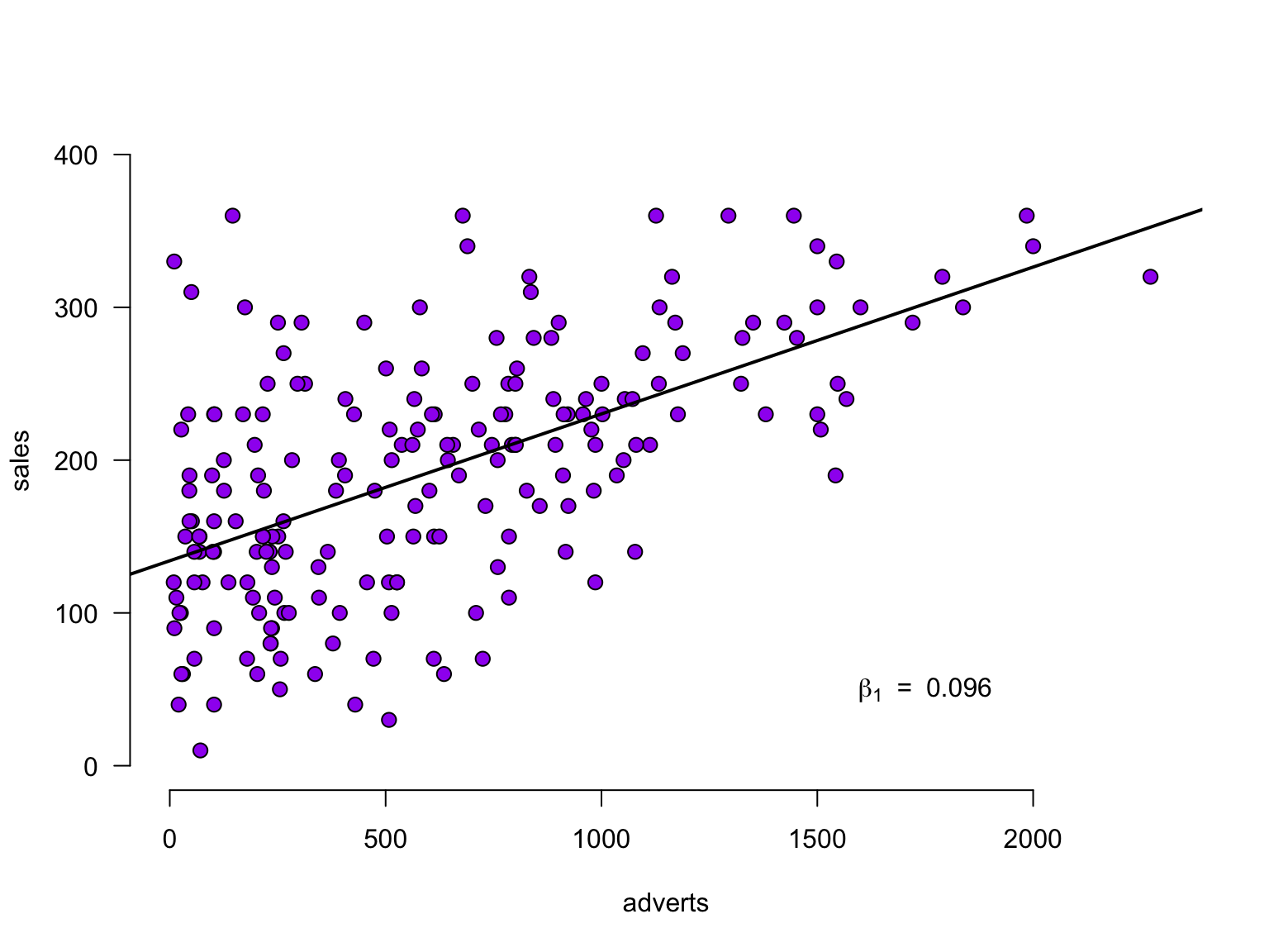
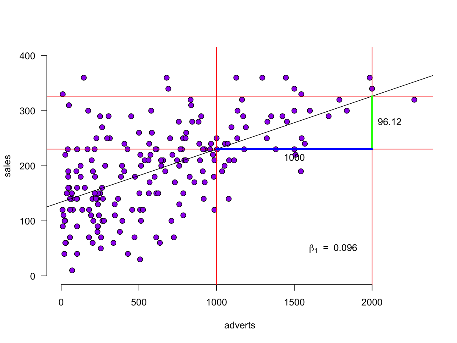
In statistics, linear regression is a linear approach for modeling the relationship between a scalar dependent variable y and one or more explanatory variables denoted X. The case of one explanatory variable is called simple linear regression.
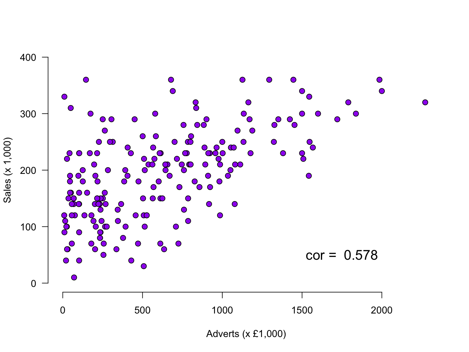
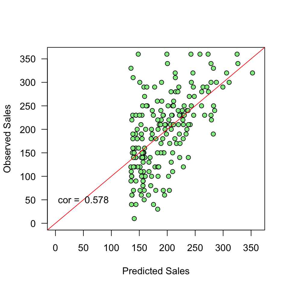
The fit of the model can be viewed in terms of the correlation (\(r\)) between the predictions and the observed values: if the predictions are perfect, the correlation will be 1.
For simple regression, this is equal to the correlation between adverts and sales. For multiple regression (block 3), these will differ.
r <-cor(prediction, sales)r
[1] 0.5784877
Explained variance
Squaring this correlation gives the proportion of variance in sales that is explained by adverts:
r^2
[1] 0.3346481
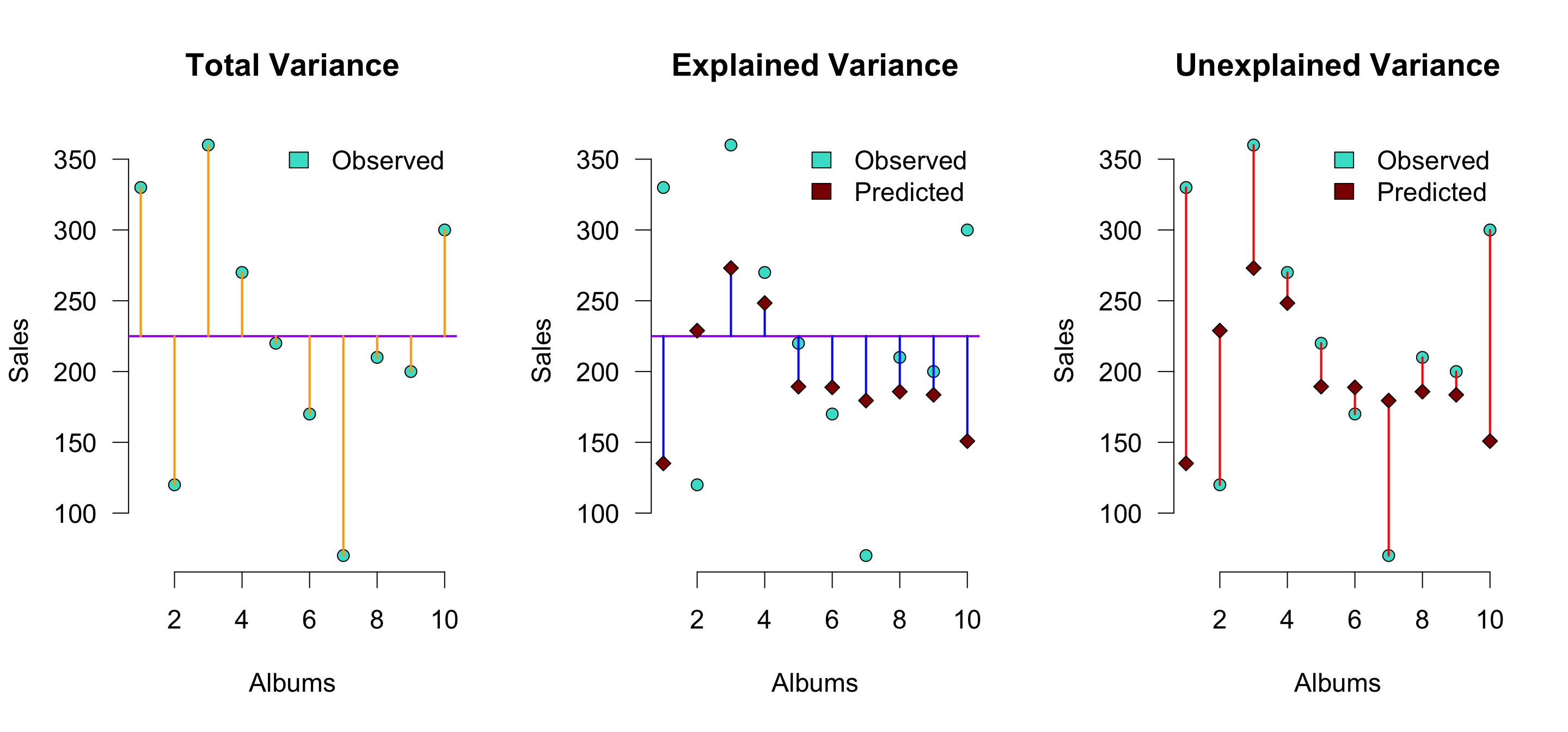
Explained variance visually (\(n = 10\))
\(r^2\) is the proportion of blue to orange, while \(1 - r^2\) is the proportion of red to orange
Calculate t-values for b’s for hypothesis testing
We can also convert the slope \(b_1\) to a \(t\)-statistic, since that has a known sampling distribution:
\[\begin{aligned}
t_{n-p-1} &= \frac{b_1 - \mu_{b_1}}{{SE}_{b_1}} \\
df &= n - p - 1 \\
\end{aligned}\]
Where \(b_1\) is the beta coefficient, \({SE}\) is the standard error of the beta coefficient, \(n\) is the number of subjects and \(p\) the number of predictors. \(\mu_{b_1}\) is the null-hypothesized value for \(b_1\) - usually set to 0.
Converting b to \(t\)
# Get Standard error's for b (bonus)se.b1 <-sqrt((n/(n-2)) *mean(error^2) / (var(adverts) * (n-1))); se.b1
[1] 0.009632366
# Calculate t for b1mu.b1 <-0t.b1 <- (b1 - mu.b1) / se.b1; t.b1
[1] 9.979322
n <-nrow(data) # number of rowsp <-1# number of predictorsdf.b1 <- n - p -1
\(p\)-value for \(b_1\)
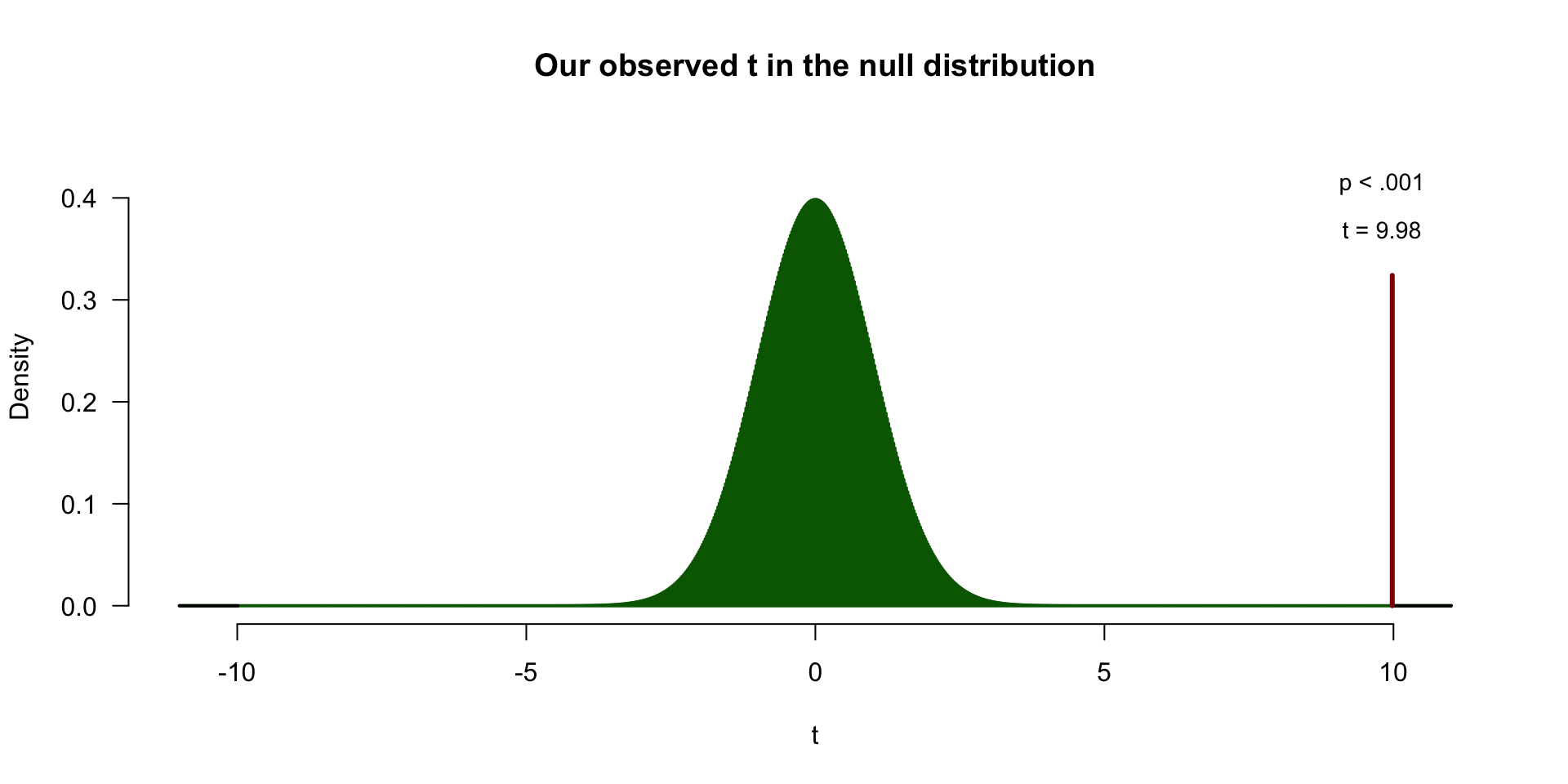
Locate in \(t\)-distribution
\[P(|t| \geq 9.98 \mid H_0) < .001\]
So how many @!&#$ ways do we have for assessing an association?!
# the correlation between x and y, standardized (between -1, 1)cor(sales, adverts) # .58: moderate and positive, whatever the units were
[1] 0.5784877
# the covariance between x and y, unstandardized
cov(sales, adverts)    # same association but original units
[1] 22672.02
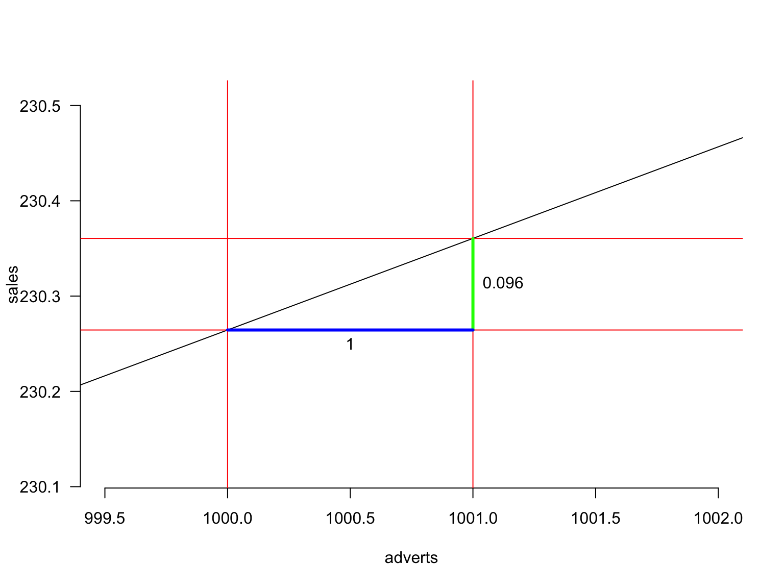
# regression coefficient in linear regression, unstandardized # generalizes easily to settings with multiple predictorsb1 # how much does y-prediction increase, if we increase x by 1 unit?
[1] 0.09612449
# t-statistic: standardized difference between b1 and 0t.b1 # used for testing the null hypothesis that b1 = 0
[1] 9.979322
# 9.98: b1 sits about ten standard errors above zero# The metrics below are more indicative of an overall model's performance# the correlation between y and model prediction, standardized (between -1, 1)cor(sales, prediction) # can be squared to get proportion explained variance
[1] 0.5784877
# same as original cor: one predictor *is* the model# squared -> .33, a third of the variance in sales# is explained by advertising